Node Based Computation

At the core of the HGraph framework is the concept of node based computation. Nodes, from the graph perspective, are the labeled entities that start or terminate a directed edge. In the computation model, nodes are the things that do work (or computations), edges describe a information flow or dependency between a nodes result and the code that depend on the results for their computation.

A node can represent a large complex computation (for example an optimisation), or a very small one (for example an addition). In HGraph the preference is to decompose the problem into a collection of small or very small operations.

The most simplistic graphs are those that are linear, that is, are a set of steps with each step leading to the next. For example:

This very simplistic graph gains very little using HGraph and could be implemented imperatively or using a simple observer pattern without and significant consequence. That said, very few graphs are simple linear lists of operations.

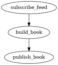
If we continue with this example we could expand the logic a bit and the graph may look a little more as below:

As we understand the requirements more fully, most real systems quickly decompose into a graph of complex dependencies.

When we have complex dependencies processing ticking data HGraph becomes very useful.

You may be wondering what a node is (from a code perspective). In HGraph a node is synonymous with a Python function.

Under the covers a node is actually a class that contains as it’s attributes the inputs to the function and the output (if present). The class then has a method called eval the gets called when the node scheduled by the evaluation engine. This function will perform basic checks to ensure the function’s pre-conditions are met, if they are it will call the function and take the result and apply it to the output (if present).

As a user though, a node is a decorated Python function. There are a number of decorators that can be used to indicate the function is in fact a node, these depend on the nature of the node you are creating.

There are three key types of nodes, namely: source, compute and sink nodes.

These have been defined in other sections of the documentation, but basically a source node introduces events or ticks into the graph, a compute node consumes ticks and produces its own ticks and a sink node will consume ticks and any further action is considered as being ‘off graph’ (or in other words once the sink node is called the graph no longer tracks the results of the node).

Source Node

The source node is split into two types of source node, namely pull and push nodes.

The pull nodes are those which know in advance all the ticks and timing of the ticks (or are scheduled by events occurring during the evaluation of a node). You may think of these are being non-threaded events, at the end of an evaluation cycle the pull nodes WILL be able to indicate when their next tick should be evaluated (or if they have a next tick to evaluate) and this will not change over the passage of time.

By contrast, the push nodes are able to introduce ticks (or events) into the graph at any time, even after the evaluation cycle of a graph has ended. In all cases a push node will be associated to a thread which is not the engines thread. These nodes are able to introduce events, in a thread-safe manner, to the graph at any point in time. As such push nodes are only meaningful when evaluated under the REAL_TIME engine.

Pull Source Node

Pull source nodes wrap data sources such as databases, dataframes, constant values and internal feedback loops.

Pull source nodes are active during simulation and real-time modes, unlike push source nodes which are only active in real-time modes.

The pull source node is exposed in the Python API using the generator decorator.

A function decorated with this decorator will be evaluated during the start life-cycle and is expected to return a Python generator which emits a tuple of scheduled time and value to apply to the output at that time. For example:

@generator
def const(value: SCALAR) -> TS[SCALAR]:
    yield MIN_ST, value

This is a very naive example, but shows the key idea of what needs to be done.

Push Source Node

The push source node provides the means to introduce ticks into the graph from external sources that are asynchronous in their nature. The push node ensures thread safety when interacting with the graph engine. As with all data in HGraph, the push source node must use logically immutable data structures to introduce data into the graph.

The push source nodes are only available to be used in real-time mode.

The exposure of the push source node in Python is via the decorator push_queue.

As with the generator in the pull source node, a push_queue wrapped function is called during the start life-cycle. It takes at least one input, the sender, as per below:

@push_queue(TS[bool])
def my_message_sender(sender: Callable[[SCALAR], None]):
    ...

The push_queue takes the output type, as a parameter, then the function is injected with a callable instance that can be used to inject events / ticks into the graph.

Typically the method will construct a thread and pass the sender to the code that runs on the new thread. But it could also capture the sender in a callback that is registered with the external data source (these callbacks are called on the external source thread, so we are still in effect ‘creating a thread’)

Compute / Sink Node

Compute nodes are the main working nodes in the graph, they consume ticks and produce results that are used by other nodes.

Sink nodes consume inputs but do not produce outputs, they can be viewed as taking ticks off of the graph.

Compute nodes, as with sink nodes, take in one or more time-series inputs. They also, unlike sink nodes, define an output time-series type. The output type holds the result of the nodes computation.

Unlike graph functions, the compute_node and sink_node function is called each time an active input is modified. It is possible to constrain, using the decorator, which inputs are to be marked as active, it is also possible to mark which of the inputs must be deemed valid for the node to be called.

Note

Where possible avoid creating your own nodes, it is best to operate at the graph level as much as is possible.

That said, there are a few times where using a compute node is a good idea, these include:

• When the atomic behaviour is not already available in the standard library.

• For performance reasons, for example when there are multiple steps in a computation that have no other dependencies, collapsing into a single node reduces the overhead.

• To have control over node activation. Doing so using graph methods can be more complicated.

The design philosophy of HGraph is to make nodes small and single purpose, with the objective of creating simple, reusable building blocks. Each block should be extensively tested and should always be designed from the perspective of the concept the node represents rather than the expected use case.

Then when using the nodes in a graph, the user can rest assured that the bulk of the testing complexity is handled and all that is to be focused on is the business logic.

An example of a compute node is:

@compute_node
def sum_a_b(a: TS[int], b: TS[int]) -> TS[int]:
    return a.value + b.value

When using a time-series in the context of a node, the value is an object which has a number of properties, one of the properties is the current value. So while a + b will work in a graph context (since this will map the code to add_(a, b), within a node you need to write a.value + b.value. For more information on the time-series types see: Time Series Types.

An example of a sink node is:

@sink_node
def write(ts: TS[str]):
    print(ts.value)

Node Scheduling

Another important consideration in node based computation, is the notion of scheduling. The graphs of nodes show dependencies, but this could be said of empirical code as well (that there is a dependency graph). In many compilers these dependencies are tracked to attempt to write out more efficient code by re-ordering operations or perform things such as escape analysis for variables inside of a loop.

In HGraph, the dependencies are used to for a flow graph of information, this is used to determine when code needs to be called and when it does not. If a node is not evaluated, then it’s results can not have been modified, thus all code dependent on the node may not need to be evaluated, this structuring allows for more efficient computation of results. The DAG produced during wiring is topologically sorted and a rank is allocated to each node, the nodes are then fully ordered. This allows the scheduler to ensure that if it processes nodes from top to bottom, that if a dependency is scheduled for evaluation (for example due to a change in a parent nodes value) that the node will not get missed.

The most common mode of scheduling is when an output is modified, this causes any nodes registered as observers of the output not be marked as scheduled for the current engine time. We discuss the common forms in which the setting of outputs can occur. This is broken down into four key types:

1. Push nodes can update their state as requiring to be scheduled, this includes updating a conditional variable to indicate that there are push nodes requiring scheduling. The timing of the scheduling is left up to the evaluation engine, when the engine is ready to process new events from push nodes it will assign it a time and cause the events to be set on the output of the push node. If the engine is in a waiting state, then this will be the current clock time, if not it will be the engine time that the engine decides to process the pull queues in. NOTE: The arrival time of the event into the push node is not considered as a scheduled time, the scheduled time is always left up to the evaluation engine for this types of node.

2. Pull nodes are scheduled based on the next event time, this is set during the start life-cycle or during the course of evaluating the graph. At the end of the cycle the next scheduled time for pull nodes is know and the graph will wait until that time is considered as now (in real-time mode) or the engine time is advanced to the smallest next scheduled time and the graph is evaluated.

3. Compute nodes will schedule dependents to be evaluated in this engine cycle (setting the evaluation time to the current engine time).

4. Compute / Sink nodes with the scheduler injectable can request that they are evaluated at a particular point in time. This will cause the node to be scheduled for evaluation at the time requested. This is the only method used to schedule a node that is not related to the using the output for scheduling the node (outside of the push and pull nodes).

The evaluation engine will cause that scheduled nodes are evaluated by moving through to the next smallest time that a node is scheduled for. This (as discussed earlier) is dependent on the mode of operation, with REAL_TIME having an active wait until it is ready to be scheduled and SIMULATION moving the time forward to the next scheduled time.

Node Activation

A node may be scheduled for evaluation, but that does not mean in will be evaluated. The compute and sink nodes are able to describe pre-conditions for evaluation, these pre-conditions include:

active

The tuple of input names that are to be marked as being active, if set to None, all inputs are marked as being active. This will cause the inputs identified to be set to the active state, this subscribes the node to the output bound to the input, causing the node to be scheduled when the output changes / is updated.

valid

The tuple of input names that are to be checked to ensure that are marked as being valid. If set to None, all inputs are required to be marked as valid. If one of the identified inputs are not valid, the function will not be called even if other inputs are valid and have been modified. Once all inputs identified become valid the function is eligible to be evaluated, this will only occur when an active input is modified. So for example, if you have two inputs, say a and b, and a is marked as active, but b is marked as valid. Then it is possible for a to be valid, but not ticking at the same time as b, so when b becomes valid, this does not cause the function to be called until a ticks again. This can be a cause for surprise in new users.

all_valid

The tuple of inputs names that are to be checked to ensure that they are marked as being all_valid. If set to None, no inputs are considered. This is similar to the valid, but the check is stronger. All valid requires that each element of the input is valid and not just any element. This is a more expensive check, ensure that it is necissary before using this constraint.

It is also possible for the user to programmatically update the active / passive state of an input, by calling the make_active / make_passive methods on the input.

Note

Making an input passive, does not stop the output associated to the input from updating its value, just stops the node containing the input to be scheduled when the value changes, thus the value associated to the input is always up-to-date.

Using the checks ensures that common patterns are handled in the framework, but it is also possible for the user to check for validity and to check which input has ticked in this engine cycle using the attributes on the time-series inputs themselves.

Marking inputs as being passive is a powerful tool to reduce unnecessary computation. For example, assume we were writing a trade acceptor, the function signature may look something like this:

@compute_node(active=("trade_request",), valid=tuple())
def trade_acceptor(trade_request: TS[TradeRequest], market_data: TS[L2Price], parameters: TSD[TradeParams]) -> TS[bool]:
    ...

In this case we need to make a determination to accept or reject a trade request, we are only interested in being called if the trade_request ticks, all other inputs are used as data to help make a decision, but we only need to make a decision if a new trade request is received. Thus we only mark the trade_request as active.

We also need to ensure we reject a trade that can’t be accepted due to missing information, so we set valid to be the empty tuple, this means that we don’t restrict calling this function if any of the inputs are not valid. Note that we don’t need to set trade_request as valid, since by definition it must be valid if the function is called (since it is also the only active input).

The logic of the function may look something along the lines of below:

if market_data.valid and parameters.valid:
    # Perform checks
    ...
    return result
else:
    return False

Notice the check for validity now performed as part of the body logic.

It is important in node based graphs to try and stop evaluation as soon as possible to reduce unnecessary computations to be performed.

Node Outputs

Since scheduling is almost always performed when an output is set, it is worth noting a few useful thoughts on this topic.

Returning None or not returning a value is equivalent to not setting the value on an output, this will leave the value in it’s last known good state and will not cause any nodes to be scheduled. So only return a result if necessary. The output WILL NOT ignore setting a value if it is the same as the current value. There are many valid reasons to reset a value. If your nodes contract states that only changes to values will be propagated, then you will need to ensure you only tick when the value is different. The easiest way to do this is to use the _output injectable. For example:

@compute_node
def de_dup(ts: TS[SCALAR], _output: TS_OUT[SCALAR] = None) -> TS[SCALAR]:
    if _output.valid and _output.value == ts.value:
        return
    else:
        return ts.value

In this example we implement a simple version of the de_dup command. This checks the output to see if it have a value, then if it does it does a simple equality check to see if this value has already been emitted. If not it will return the value it received, otherwise it is returning a None value. For the _output injectable the type does not care what the type is, but it is nice to use the _OUT as it provides more context support in the IDE.

Using REF to reduce activations

Another tool to reduce necessary activations of nodes is the make use of REF time-series types. The reference type ticks references to an output rather than the values of an output. This can be used when the value of the input is not required, for example:

@compute_node
def select(condition: TS[bool], on_true: OUT, on_false: OUT) -> OUT:
    if condition.value:
        if on_true.ticked or condition.ticked:
            return on_true.value
    else:
        if on_false.ticked or condition.ticked:
            return on_false.value

This is the base case where we use normal inputs, in this case the select function will be evaluated if any of the inputs tick and will produce a result based on a combination of the value of the condition and if the input associated to the condition ticked or the condition ticked.

The current version of the function will be evaluated as often as the inputs tick, this is wasted when the ticked value is not going to be processed, but also, there is no need for the function to know the value of the on_true and on_false inputs. In this case the function is prime to benefit from using the REF type, this is the refactored version:

@compute_node
def select(condition: TS[bool], on_true: REF[OUT], on_false: REF[OUT]) -> REF[OUT]:
    if condition.value:
        if on_true.ticked or condition.ticked:
            return on_true.value
    else:
        if on_false.ticked or condition.ticked:
            return on_false.value

On first pass there seems to be very little different, the logic looks the same, the only difference is the change to the on_true, on_false and output types. The difference is in the activation of the code, the code will now activate when the condition ticks, but will be additionally activated if the output associated to the on_true or the on_false inputs change, that is not when the value of the outputs change, just when the output pointed to by the REF changes. This typically does not happen often, especially if the source passed to this code is the output.

This can make a significant change in how often this node is activated.

This pattern is useful when working with logic that manipulates the selection of time-series, but does not depend on the actual value. Operations that benefit include:

• Pivoting time-series (such as TSD)

• Selection of TSD values based on keys

• Manipulation of TSB values such as modifying an individual element or selection.

References do add complexity to debugging as the ultimate consumer (dereferenced input) becomes connected to a part of the graph that may not be immediately obvious from the code.

References are used extensively in library code so being aware of them and how the work is important to debugging graphs.

Tracing issues

Graph programming changes how we can debug code, the advantages of modularity and the powerful mechanisms introduced to manage change come with some complications in debugging. These complications are not very different from code using messaging systems or other event based architectures, but the fine grained nature of the nodes can make this problem more tricky to handle.

HGraph attempts to make debugging the graph as easy as possible, here are some typical debugging problems and tools in place to assist with identifying the issues.

IDE / Python debugger

Code in nodes can be break-pointed, that is if you are trying to figure out what is going on in a node, then you can use standard Python debugging tools. By placing a breakpoint in the node you can inspect the code in the function as well as navigate from input to outputs (traversing the graph). This can allow you to see the value of nodes that are in the preceding tree of the node you are debugging.

There is no callstack of nodes though, once a node is evaluated, all there is is the value it produced.

Trace

Sometimes the node you are expecting to be evaluated is not evaluated, this means that it is not possible use a break-point to see what is going on, in this case using the trace options in the graph runner config can be very helpful. This will dump out the evaluation trace of the graph as it gets evaluated. It will display information such as which functions are evaluated, what the input values were, which inputs were ticked, etc.

The output from this tool can be very large as it is very details, so this is recommended mostly for small apps, or by filtering to hit specific paths through the graph. This is suitable for debugging test cases where the code can be limited to a reproducible test case as well.

Introspector

If you are working with a large real-time graph, then you will want to use the introspector to be able to perform inspection of the live running graph, this tool allows you to see all of the nodes, their current state, as well as chart performance and latency of the graph.

The tool allows for live inspection of the graph, this is helpful tracing down issues such as; “Why did my not not tick”, “What is the state of nodes around the node of interest”, as well as performance related issues.

This is more intrusive and requires you to wire the component into your graph in order for this functionality to be available.

For more information see HGraph Inspector.