Time Series Types

The time-series types define the ports of the node that allow the graph to be connected. A node in the graph is allowed at most one output port. This port can be connected to zero or more input ports. The flow of information is from output to input.

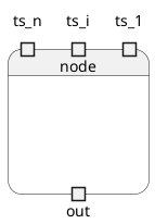
$@startuml state node { state ts_1 <<inputPin>> state ts_i <<inputPin>> state ts_n <<inputPin>> state out <<outputPin>> } @enduml$

Non-time-series inputs are supported as inputs, these define the configurable properties of the node and do not change over time. We refer to these as scalar properties to indicate that they do not have a time-dimension.

We distinguish input and output time-series types. Input time-series properties can be connected to output’s. The output time-series type holds the value of the time-series property, the input time-series type references the value in the output type.

Another way of thinking about the time-series properties is to think about them in terms of the observer pattern, here the output can be viewed as the observable and the input the observer. The observable holds the source of information and the observer is associated to the observable, in this case (as with property observers) it can see the value and will be notified when the property changes.

The other way to think about this is using the pub-sub pattern, the output is the publisher and the input is the subscriber. As with classical pub-sub, there is a single publisher for a topic (or property) and zero or more subscribers to the property.

An output time-series value can be set, but an input time-series value can only be read.

Using the HGraph model, input time-series’ are declared as function arguments and output time-series values are declared as return values.

Thus, when calling an HGraph function, (if it has a return type defined) the value returned (when using the graph decorator) is a reference to the output port of the graph (or the time-series output).

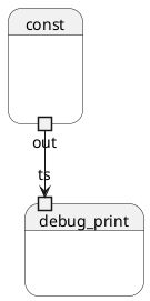
Let’s consider the following code:

@graph
def my_example_graph():
    c = const("world")
    debug_print("hello", c)

In this trivial example, c represent the output time-series of the const node. "world" is a scalar input defining the configuration defining the value that the node will tick with. debug_print is connected to the const node by passing c to the time-series input of the node. Creating the graph:

$@startuml state const { state out <<outputPin>> } state debug_print { state ts <<inputPin>> } out --> ts @enduml$

Time-series properties

The time-series types have the following properties:

$@startuml class TimeSeries { owning_node: Node owning_graph: Graph value delta_value modified: bool valid: bool all_valid: bool last_modified: datetime } @enduml$

The time-series type is aware of the node it is bound to. This can be extracted from the owning_node property. This is most useful when debugging the graph, but generally is used more for framework code (as is the owning_graph).

The owning_graph property declares the graph the node belongs to, this is the runtime graph, not the wiring graph.

All inputs are capable of presenting their current value state as a Python object. This is accessed through the value property, the delta_value property is also a Python representation of the time-series, in this case it represents the change in value. This is only really useful on complex types, such as a time-series collection class, where the delta represents the elements that were modified in this engine cycle. Whereas the value property represents the current valid values of the time-series, which include results that have previously been modified / set.

There are two useful flags associated to the time-series, modified and valid. Where modified is True if the time-series type was modified in the current engine cycle and False otherwise. The valid flag is True when the value has been set at least one, or in other words, has a valid value associated to it. Note, there are circumstances where a value can transition from valid to invalid, so the naive statement of at least set once is not 100% true.

The all_valid flag is True when all inputs / outputs of a collection type are valid, for example in a TSL (time-series list), it is possible that only some of the elements in the list could be valid and others not yet valid. The all_valid property ensures that each input is valid. This is a stronger requirement then valid which becomes true as soon as at least one element becomes valid. Checking for all_valid is potentially a very expensive operation and as such should only be used when this constraint is actually required to be enforced.

Finally, the last_modified time represents the time this time-series value was last modified. This can be useful for a number of reasons, but a simple use-case is to deal with staleness checking of a value.