HGraph: Functional Reactive Programming in Python

Abstract

HGraph is an implementation of the Functional Reactive Programming (FRP) paradigm in Python. This document provides a description of FRP, how HGraph implements FPG and how the implementation matches the FRP model.

Introduction

Functional Reactive Programming (FRP) is a programming paradigm that combines functional programming with reactive programming. The landmark paper describing this approach is “Functional reactive animation” [Elliott and Hudak, 1997]. In this paper, the authors describe a functional approach to coding event/time based logic. Their focus was on the generation of animations, but the concepts are applicable to any time based system. The key concepts from this paper can be summarised as follows:

Events: These are first class values and the instigators of change in the system. Events can contain data, and represent external stimuli that can be used to trigger changes in the system (such as a mouse click). Or internal stimuli such as a timer, parameters changes, etc.
Behaviours: These are time varying values (often capable of representing continuous time values). The example given is a collection of images over time can be viewed as a behaviour. Another example could be a point in motion, where the point is defined by a set of coordinates over time. The value of the coordinates could be computed at any point in time, thus the behaviour can produce a scalar (with respect to time) value given a point-in-time.

The paper goes on to describe how to use these concepts to produce animations using Fran (Functional Reactive Animation). This is a functional language built around the event and behaviour concepts. Time is another key element of the system.

When defining Fran, the authors introduce some interesting concepts, these include items such as lifting, time, event handling, and reactivity. This is covered in more detail later.

There have been further refinements to the FRP model, of interest is the paper “Functional Reactive Programming, Refactored” [Perez et al., 2016]. This paper provides a summary of earlier papers that provide additional classification of FRP models and covers Yampa, a Haskell based FRP model.

In this paper, the concept of events and behaviours is re-cast in terms of signal and signal functions.

Signal: A signal is a viewed as a function that maps time to a value. A signal is a stream of these values over time. This can be viewed as a time-series of values of some specific type. The signal is an input to signal functions. This most closely models the concept of Events as describe previously.
Signal Function: A signal function is a function that takes a signal as input and produces a signal as output. This is similar to the concept of Behaviours. The signal function can be viewed as a transformation of the input signal/s to produce one or more output signals.

The modes of FRP are broken down into two main branches, namely Classic and Arrowized FRP [Nilsson et al., 2002]. Where classical FRP is defined much as in [Elliott and Hudak, 1997], and Arrowized FRP is defined as a graph of causal functions (where the result of the function at time $t$ is as a direct consequence of it’s inputs in the range of $[0, t]$ ). In Arrowized FRP time is considered to be monotonically increasing. The example of “wires” to represent signals and “components” to represent signal functions is used to describe the system. Where the wires connect the boxes together and the arrow represents the flow of information.

Finally, external events are found on the outer edges of the graph formed by the signals and signal functions.

HGraph is a Python implementation of the FRP model. It could be classified as an Arrowized FRP model. It uses the term time-series to represent the concept of signals, and nodes to represent signal functions. HGraph has the concept of time being abstracted into a system wide clock that abstracts the system from the computers system clock. This allows for time to be precisely controlled and simulated.

The current FRP implementations are generally implemented as pure functional languages or within a pure functional language (such as Haskel). HGraph leverages off of the mixed model of Python, which supports functional programming but also can be used to implement imperative programs, to provide a more gentle introduction to the world of functional programming.

Functional Programming

Functional programming (FP) emphasises the following key characteristics:

Immutability of values
Use of functions to implement logic
No side-effects (in functions)
No explicit support for traditional control flow operators (such as if/else and while loops)
Declarative

Functional languages can be broken down into two main types, namely pure functional with examples such as Haskel, or hybrid languages that support both functional and imperative styles such as Python, Scalar, OCaml, etc.

As a contrast imperative programming is characterised through the specification of the steps that the computer must perform to compute a task. It makes use of variable assignment for state modification and uses control primitives to direct the flow of evaluation. The classic example of these types of langauge are C and Pascal.

With FRP being functional in nature, HGraph uses the functional aspects of the Python model, thus there are no classes (with the exception of specifying data classes). Extension of behaviour is achieved through composition and by using functions as values. Non-time-series values are considered as immutable. Behaviour should have no side-effects, etc. With signal functions being considered as causal we can view these as immutable as well (although in this case the immutability is with respect to a time-range).

The remainder of the paper focuses on specific concepts and operators described in the various papers referenced and how these concepts are implemented in HGraph.

Primitives

Time

Time is a fundamental aspect of the FRP model, behaviours / signal functions are values over time and the current time implies the current value of the behaviour. In HGraph time is considered to be discrete, and monotonically increasing. The quanta of time are expressed in the constant MIN_TD which is the smallest unit of time the engine can increment the clock by. This is currently limited to 1 micro-second due to the use of Python as the Domain Specific Language (DSL) embedding language.

There are also a minimum time and and a maximum time (MIN_TD and MAX_TD respectively). The minimum time is the smallest time we can represent. This gets set to the UNIX epoch (1970-01-01 00:00:00) as the runtime engine is ultimately to be written in C++ and the conversion between Python and C++ is done using the C ctime conventions. This results in 0 being the smallest time value and it maps to the UNIX epoch. The maximum time is set to a value in far in the future. These constants define the operational range of the engine times. These are extracted into constants as they are intended to be implementation specific and can vary.

There are a number of perspectives on time, these include:

Evaluation Time: This is the time of the event/s that are currently being processed. All signal functions are considered to have the time of the evaluation time for the consequences computed as a result of the event/s being processed. This is the clock that drives the evaluation of the program. It is guaranteed to be monotonic. It could in theory run ahead of the computers clock (when processing events in rapid succession, where the cost of computation is less than MIN_TD. But, generally runs slightly behind the system clock.
Wall Clock Time: This is logically the time of the system clock. The wall clock time and evaluation time are similar but differ based on the computation overhead and any other delays experienced between the event being accepted and the processing of the event. We refer to this as lag. The wall-clock time may not actually reflect the computers system clock, unless the program is running using the real-time engine. In simulation mode the wall-clock time is simulated to be the time of the event plus any computation overhead. This clock can be non-monotonic in simulation mode.
System Clock Time: This is the time of the system clock, i.e. the computers internal measure of time. This is never directly exposed to the programmer and should never be accessed in an HGraph application. Doing so will result in undefined behaviour. Time should always be accessed via the HGraph API.

In HGraph the clock is exposed by the abstraction EvaluationClock. This can be obtained in a variety of ways, these are covered in the main documentation set.

Evaluation Cycle / Wave: This concept refers to how events are processed in HGraph. Events are co-ordinated for delivery by time. All the events that occur within the granularity of a MIN_TD are processed together. All signals and signal functions produce a directed acyclic graph (DAG). The consequences of an event are processed until we reach the leaf of the DAG (referred to a sink node). Once all consequences are processed we consider the computation done and refer to this as a wave or an evaluation cycle. At the end of the cycle the evaluation time is incremented and the next wave is started. Where the next evaluation cycle is the time of the next smallest event time.

Time-Series

The term time-series is used to represent the concept of a signal in the Arrowized FRP model. A time-series is represented in the model however and provides the ability to describe the nature of the signal as well as providing an application programmers interface (API) for accessing the attributes of the signal from within a signal function (or node).

There are a number of different time-series types implemented in HGraph, these model the FRP equivalent of normal data types. Note that all value’s (non-time-series) in HGraph are expected to be immutable, only the time-sieres types can change over time. The time-series types are:

TS: This is the most basic time-series type and represents a stream of values over time. Much as is described in the previously mentioned papers. In HGraph the type is fully expressed as TS[SCALAR], where SCALAR is the type of the values represented by the signal. Examples of SCALAR values include int, float, str, etc. This is the time-series equivalent of a value.
TSS: This is a the equivalent of a set in FRP. It describes the change in values of a collection of values over time. The constraint being the values must be hashable. As HGraph is a typed extension, the full form of this is: TSS[SCALAR], where SCALAR is constrained to be a hashable type.
TSL: Representing a homogeneous collection of time-series signals. This is the equivalent of a list in FRP. The full expression of a TSL is TSL[TIME_SERIES_TYPE, SIZE], where TIME_SERIES_TYPE represents any valid time-series type and SIZE is the number of elements in the list, due to the restrictions on generics in Python this value must be a type and so if we wanted to expressed a list of 2 time-series we would express that as: TSL[TS[int], Size[2]].
TSB: This is a heterogeneous collection of time-series signals. This is the equivalent of a class or struct in FRP. The full expression of a TSB is TSB[TS_SCHEMA], where TS_SCHEMA is a class describing the schema of the bundle.
TSD: This is a dictionary of time-series signals. This is the equivalent of a dictionary in FRP. The full expression of a TSD is TSD[K, V], where K is the type of the key (e.g. str) and VALUE_TYPE is the type of the time-series value, for example: TSD[str, TS[float]]. This is the only dynamically sizeable type in the system. It supports the dynamic addition and removal of time-series signals.

These describe the basic wires that can be used to connect the components of the system together. There are a few additional types that represent more advanced time-series parallels to traditional typing. Namely:

REF

This behaves in a similar fashion as a pointer or variable reference. It holds a reference to a time-series signal, but does not have access to the value of the signal. To use this any of the standard time-series types can be wrapped with this, for example: REF[TS[float]]. When this is used to describe the type of an input or output, the time-series is passed by reference and not value. However, unlike a pointer, there is no standard deference operator. Instead when a reference is to be de-referenced it is passed to a node that does not indicate the input type is a REF. The library will automatically de-reference the value at this point.

REF is generally used by framework developers as a performance enhancement. Specifically when the value of a time-series is not required to be inspected as part of the behaviour implementation.

TSW

This provides a standard wrapper over a buffered time-series. This provide history of the previous states and times those states were valid. This is useful for implementing rolling window operations.

Nodes

Nodes are the equivalent of signal functions or behaviours discussed earlier (or at least these are the equivalent to a signal function primitive). HGraph is, as mentioned earlier, implemented as a DAG. Thus graph terminology is also usefully applied. The signals (or time-series) provide the edges and associated flow direction of the graph and the signal functions (or behaviours) provide the nodes.

Using graph semantics, there three types of nodes in any DAG, namely source, intermediate and sink. Source nodes are the entry point to the graph, these are the nodes that introduce events into the graph. Intermediate nodes have input edges and output edges and are connected to either source nodes (or other intermediate nodes) as inputs and sink nodes (or other intermediate nodes) as outputs. Sink nodes are the exit point from the graph, these nodes are the final consumers of the graph computations. These most often represent exporting of events to external destinations, in the simple case to a storage system, or display.

Since the DAG represents a computational graph, we use the term compute node to represent the intermediate nodes, given this to be the expected behaviour of this node type.

Source Nodes

These are the points of entry to the graph, source nodes are responsible for collecting and formatting events into time-series values. A source node has no time-series inputs in it’s definition but does have a time-series output. These nodes act as the translator between event and signal. Source nodes are the only nodes that can introduce events into the system. Source nodes are also generally defined on the outer wiring of the graph definition providing a clean separation of IO and logic. Once again, as per Arrowized FRP, this provides the ability to more easily simulate runs with the same inputs to the core behaviour and get the same results (as a consequence of the causal nature of compute nodes). In HGraph, there are a couple of ways of specifying source nodes. This include the use of the generator or push_queue decorators. Application logic should never be encoded in a source node.

Compute Nodes

Compute nodes are the work-horse of the nodes, these perform logic on time-series inputs and the results are emitted as time-series outputs. Compute nodes are expected to be primitive operations that can be composed to create functional applications. A compute node can be created using the compute_node decorator. As a guiding principle, user of the library should not generally need to create new nodes, the desire is that libraries of these nodes should exist and new applications are developed by wiring these nodes together to achieve the desired application logic. Compute nodes should never have side-effects. These represent the concept of the signal function.

A compute node is not composable, this is a primitive in the HGraph eco-system. A compute node can accept scalar functions as inputs, but not graph functions (described later).

Sink Nodes

As mentioned earlier, these are the leaves of the DAG and are, by design, allowed to have side effects. These nodes can produce events for other systems, capture the values of the time-series to storage, display items on the screen or otherwise turn the time-series inputs into something useful. These can be though of time-series to real-world adaptors. Applications logic should never be encoded in a sink node.

Wiring

Finally, we need a mechanism to assemble an HGraph application. We have the time-series types to describe the connections between nodes, the nodes to perform the logic as well as introduce and exit events from the application. But, the most important aspect is describing the flow. For this we use the concept of graph.

Graph

A graph describes the construction of a DAG (or a fragment of a DAG). It contains the definitions of how the nodes are to be connected. A graph is created by decorating a Python function with graph. When evaluated, this will be called by the graph builder function (prior to graph evaluation) and will process the connections and build the desired application graph. A graph has the same signature used for nodes, but unlike nodes, can be composed. In this sense the graph represent the true FRP function (or signal function or behaviour). Once the logic in the graph has been evaluated, the result is used to create a graph builder, which will be requested by the runtime to create a new graph for evaluation. The function decorated by graph is thus only evaluated prior to the evaluation of the DAG described in this function.

A graph is composable. A graph can be passed as a value to a graph and used within a graph. That is graph functions are first class values within HGraph (within the given constraints).

Runtime

HGraph applications are split into the declaration of logic and the evaluation of the graph described by the logic. This is separation is described as a separation into wiring logic and runtime behaviour. The wiring logic is what the application developer specifies, the runtime behaviour is the logic supplied by the HGraph package to evaluate the graphs.

The runtime consists of a graph-builder, that evaluates the functions decorated by graph and builds a DAG, this DAG is ranked and converted into a builder graph. The builder graph is used to generate out the runtime node instances that are evaluated. The final step is the run-loop, this is the logic that controls the order of evaluation of the nodes and the time of the evaluations.

There are two main runtime engines provide, namely simulation and real-time. The simulation engine evaluates the graph using compressed time, that is the evaluation clock is advanced to the next event time as soon as the last evaluation cycle is completed. The real-time engine attempts to keep in sync with the computer clock. Thus if the next evaluation cycle is scheduled for a time in the future (from the perspective of the computer clock) the engine will wait until the computers clock matches the next evaluation time before processing the next event. The real-time engine is the only engine that can process real-time events (such as network traffic, user inputs, etc.). The simulation engine is suitable for simulating events using pre-defined event streams.

Operators

This section focuses on the API and syntax of HGraph. The core language has a number of operators that are defined to assist with building basic functionality.

To start with, consider the core operators or concepts described in “Functional reactive programming, refactored” [Perez et al., 2016]. Below is how these concepts map to HGraph.

Lifting

This applies a provided scalar (or normal) function point-wise to each tick on the time-series. In HGraph we have the lift operator that performs this operation. The concept of lifting allows for re-use of existing functions within the FRP model. This is a useful tool to make existing standard Python functions available to HGraph.

Along with this concept, HGraph also provides a lower function that will convert an HGraph FRP function to a standard Python function, allowing the function to be called by traditional Python code. The time-series inputs require a Polars [Developers, 2025] DataFrame to be supplied and the result is returned as a data frame as well.

Widening

In this example we are shown how to affect a sub-component of a time-series collection. With the type system supported by HGraph, this is a relatively easy operations, using the example in the paper, we could model the inputs i: TSL[TS[int], Size[2]], then the logic would be something to the effect of: result = convert[TSL](i[0], i[2]+7). In this case the result would contain the value (untouched) of the first element in the time-series and the second element having seven added to it. There are many other examples using TSB for heterogeneous collections or TSD for dynamic collections. A feature on the time-series collection API’s (only available during wiring) is to use the copy_with method on the time-series object. This allows for pass-through of all non-over written values and replacing the values supplied. This is a very efficient operation as the cost is only born during wiring, not evaluation.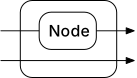

State

State in FP is often implemented using recursive definitions, given HGraph is evaluated as DAG, this is problematic. We require evaluation of a wave to be directional and acyclic. Thus it is not possible to compute a recursive value at point $t$ in time. To overcome this we have a couple of options provided, the first is to use a concept of feedback, this is similar to that discussed in section 3.5 by Parez, et. al. 2016. This creates a recursive relationship where the cycle is broken overtime. With the result been returned to the graph on the next smallest time-interval (MIN_TD).

The other mechanism for state, specifically in the case of the compute_node or sync_node, is using the concept of injectable attributes. This a mechanism to declare a need to track state, then the runtime engine provides a state object to the function. This is logically a shortcut for using a feedback, but also allows for mutable values to be stored on the state object. The state is provided to the function and as a consequence the function itself is stateless, and any state can be provided to the function, although in actual use, the state is effectively a dictionary that is provided to the function on each activation.

Constant

In the FRP, a constant is a value that is held continuously from a point-in-time and never changes thereafter. The const operators performs this function in HGraph, the const operator emits the value provided at the first time possible in the runtime of the graph. This is usually the start-time, although in the case on nested graphs, this is the start time of the sub-graph and not the outer graph. Each time-series type can be expressed as a constant.

Arrow

Next we consider the paper “A new notation for arrows” [Paterson, 2001], whilst a number of the concepts previously discussed are already derived from this paper, there a few few concepts that are worth expanding on. This paper presents an extension to the Haskell to better support monadic computation and expression of the computation. Whilst HGraph itself does not enforce monadic computation, there are a number of scenarios where the approach could provide more readable code.

The arrow approach can be re-expressed using Python as follows:

There is a function that will wrap a standard function (monoid) providing the ability to make use of the new arrow syntax. For example:

class Arrow(Generic[A, B]):  # Where A, C, C, D are TypeVar's
    def __init__(self, func: Callable[[A], B]):
        self.func = func

    def __rshift__(self, other: 'Arrow[B, C]') -> 'Arrow[A, C]':
        return Arrow(lambda x: other.func(self.func(x)))

    def __call__(self, value: A) -> B:
        return self.func(value)

def arr(func: Callable[[A], B]) -> Arrow[A, B]:
    return Arrow(func)

def first(fn) -> 'Arrow[tuple[A, D], tuple[B, D]]':
    return arr(lambda pair, _fn=fn: (_fn(pair[0]), pair[1]))

This adds support for chaining and dealing with tuples, for example:

mul_2 = arr(lambda x: x*2)
add_5 = arr(lambda x: x+5)
(mul_2 >> add_5)(3)

>> 11

to_upper = arr(lambda x: x.upper())
first(to_upper)(('hello', 42))

>> (“HELLO”, 42)

With these primitives defined, a small set of utilities are described to build out the core operator set.

swap = arr(lambda pair: (pair[1], pair[0]))

def second(f: Arrow[B, C]) -> Arrow[tuple[D, B], tuple[D, C]]:
    return swap >> first(f) >> swap

def assoc(pair):
    (a, b), c = pair
    return a, (b, c)

def cross_over(f: Arrow[A, B], g: Arrow[C, D]) -> Arrow[tuple[A, C], tuple[B, D]]:
    # In the paper this uses *** as the operator
    # Allowing f *** g to be used
    return first(f) >> second(g)

def fanout(f: Arrow[A, B], g: Arrow[A, C]) -> Arrow[A, Tuple[B, C]]:
    # Uses &&& in the paper allowing for syntax such as f &&& g
    return arr(lambda b: (b, b)) >> cross(f, g)

def apply(pair):
    return arr(lambda pair: pair[0](pair[1]))

This approach provides a interesting way to describe the flow of information.

HGraph supports this model with with the hgraph.arrow module.

A few small differences exist, namely first and second are selectors to select the first and second tuple elements from a pair. The // operator is use to implement the cross_over function and / is used to implement the fanout operator. Finally, since HGraph is strongly typed, and there is already an apply function, apply_ is provided, it takes the output type of the function as a parameter.

As can be seen HGraph lends itself well to the ideas expressed in the current body of work describing FRP and can be adapted for follow alternative composition strategies.

Flow Control

For programmers with an imperative programming background, the lack of flow control keywords and structures in FP can be a bit daunting, this can be even more interesting when dealing with reactive flow control. There are a number of strategies for different froms of flow control, these include:

Recursion: Instead of using loops, recursive functions can be used to implement looping. There are many strategies to manage the cost of recursion, the key one being tail recursion, where the final computed value is returned, directly. This avoids the requirement of tracking the call-stack to support unwinding. In FRP, recursion is not generally the approach taken, however, the use of the feedback operator allows for the simulation of general recursion. There are a number of other related operators to support processing in a similar manor, for example there is the emit operator, which takes a collection and emits that values one element per evaluation cycle. These strategies spread the recursive operations over multiple engine cycles.
Higher Order Functions: These functions take other functions as arguments and provide the ability to implement common control flow patterns. In the paper “Monoids for functional programming” [Wadler, 1995] there in an interesting introduction to some of these ideas, albeit in a monoid form. Whist HGraph can support monoid operations, it is a hybrid langauge and as such generally uses a more conventional calling approach, however, the concepts discussed are found in HGraph as well. The include: map_, reduce, filter_, as well as a number of other constructs.
Pattern Matching: Matches the structure or content of the data. HGraph supports two key concepts to support this behaviour, namely: switch_, operator, and dispatch. The switch_ is a higher order function that performs a similar function to the switch keyword found in many C like languages. The function takes a match time-series that contains a value that will match a key in a dictionary. A dictionary of matches and associated FRP functions to apply when the match is achieved, and any parameters to supply to the matched function. The operator is a wiring time matching function. This will match the wiring time type and scalar information selecting the implementation that is the closest match. This is equivalent of polymorphism in imperative programming. Finally, there is the dispatch higher order function, this is a hybrid technology in that it relies on matching the type of the input data to the closest sub-class of the defined input type. This is similar to traits in Rust or virtual dispatch in C++.
Continuation-Parsing Style (CPS): This is discussed in “Representing Control” [Danvy and Filinski, 1991]. In simple terms, this deals with asynchronous or complex control flow (such as exception handling) by using a function to apply when the condition occurs. In FRP asynchronous behaviour is handled as base functionality of the system, however, exception handling is an interesting challenge. HGraph provide an approach more consistent with that described by Wadler 1995. Where the exception is provided as a separate time-series stream, normally not visible, but accessible using the exception_time_series function. This allows for logic to be bound the the time-series as standard logic. It is also possible to bound a sub-graph of behaviour using the try_except higher order function. This effectively wraps the nodes with a large try-catch block and the error result is provided on the exception output key and the non-exception result on out.
Other Abstractions: HGraph provides a number of other higher order functions to support other concepts, for example for if/else can be simulated using the if_then_else function, which will select a time-series stream based on a condition, this can also be simulated using a switch_ with True and False matches. Another approach would be to use the if_ operator, which will direct a time-series flow down the True or False output keys depending on the value of a condition time-series.