Mental Model

HGraph defines a DSL (Domain Specific Langauge) using Python as the hosting language, and whilst every attempt is made to make the code look and feel like Python, there are a few key elements that differ from standard Python programming. These differences will require a change to how things are done from standard Python and require a change to the mental model when writing code. Below are some of the key concepts or ideas that drive the HGraph mental model:

• Graph

• Time-series

• Functional

• Typing

The rest of this section attempt to introduce these concepts.

Graph

Graph evaluation is a conceptual approach to describing the relationships between different elements of the program and how information flows through the code, there are a number of different approaches to this, but most models focus on the concept of a DAG (Directed Acyclic Graph).

Backward Propagation Graphs

In a DAG information flows based on the directed edges and the nodes represent a computation that is applied to this information flow. Under this model there are two approaches to implementation, in the first model (referred to as backward propagation graphs (BPG)) the user requests a node to be evaluated, and this causes the model to traverse the dependencies of the node evaluating those nodes that require it and then finally produce a result. This is the model used in spread sheet applications.

For example, consider the cells in a spread sheet with values and formulas below:

A1 = 5
A2 = 2
B2 = A1 + A2
C2 = B2 / A1

The the DAG for this graph is:

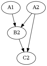
Whilst the graph shows information flow from A1 to B2, etc. In it’s use, data is requested from leaves of the graph, thus if the user selects C2 and requests the cell to be evaluated, the requested will logically bubble up to B2, which need to be computed, so the request bubbles up to A1, this is a value cell so no computation required, then the cell A2 is requested, it too is a value cell so the result is available. B2 has all of it’s dependent properties evaluated so B2 is now evaluated, the finally C2 will check A1, this is ready so C2 is now evaluated and the computation cycle is over.

There are variations on the exact algorithm used to compute the values in the dependent nodes, but the they are all logically the same as described above. The other trick that a backward propagation graph plays is remembering what it has already computed, to do this the graph will notify children when the cached value is no longer valid. This is done by marking children as being invalid. Thus if A2 were modified, it would mark B2 as being invalid, B2 would then mark C2 as being invalid. Thus when the user requested the value of C2 again it would require the re-computation of B2 and C2.

In complex graphs, a small change to the overall computation can ensure that only a small amount of re-computation is required to evaluate the graph.

This model of computation is really valuable when only selected leaves are required to be evaluated or the user is experimenting with small tweaks to the values that are made in multiple steps before re-computing the results.

Ad-hoc what-if analysis is a good example of where this style of computation can be useful. There are really advanced versions of this model that can provide additional concepts such as computation layers to improve scenario analysis.

The model was a great solution in days past, however, in most modern use-cases this model is less efficient, especially in scenarios where users wish to immediately see the results of data changing. (For example auto-recalculate in modern spread sheet applications).

The problem with the backward propagation model is the invalidation logic, when properties change invalidation is expensive, especially if then end result is just to re-compute the leaves. This also requires additional mechanisms to be added to be able to subscribe to cell invalidations in order to be able to request a re-compute.

Forward Propagation Graphs

At this point we introduce the forward propagation graph (FPG). This graph is similar to the backward propagation graph, in that it is a DAG, the information flow is from source nodes, to sink nodes (leaves), but in this model information changes cause an immediate re-computation of the graph.

Additionally the user does not request a node to be computed, when information changes at one of the source nodes, the graph computes all dependent nodes and all leaf values are always re-computed (if necessary).

This avoids the invalidation / request cycles in the backward propagation graph. It does have the weakness that all values are computed whether or not they are required. It also means that many small changes over time will cause multiple computation cycles to occur. Thus additional work is required to mitigate these issues if required, whereas they would be free in the BPG.

In both graph styles evaluation of nodes ensures that a node in the graph is only ever evaluated once for a given change. In the FPG graph, the evaluation is typically performed by evaluating nodes in rank order, where the rank of a node is determined by it’s topological ordering.

Observer Pattern

A way of thinking about the FPG is in terms of it’s primordial ancestor pattern, the observer pattern.

In the basic observer pattern, we have an observable and one or more observers.

In the example above, the observables are the cells, the observers are the cells with dependencies. That is, A1 and A2 are observables, B2 is observable and observer (observing A1 and A2) and C2 is acting as an observer (of B2 and A2).

If we followed the traditional observer pattern, when A2 is modified it will notify (wlog) B2, which will re-compute it’s value, then it will notify C2, which will re-compute its value. Then A2 will notify C2, causing C2 to be recomputed again.

This is a real problem, we have two negative consequences:

1. C2 has been evaluated twice (more computation than required)

2. C2 may have an incorrect interim result (inconsistent state)

These are not acceptable outcomes, thus the basic observer model is not suited for complex event based computations.

The FPG extends the observer pattern by separating notification from evaluation.

In the FPG model, the dependent nodes (or observers) register as observers, but instead of the eval() method being called in the event dispatch loop of the observable, we add a new component, the scheduler, which is instead notified that the node should be evaluated. The the scheduler performs the call to eval(). This allows the scheduler to ensure that the order of evaluation ensures that a node is only evaluated once all it’s ancestors have been evaluated. This ensures we only evaluate the node one for a given change set and the results will be consistent.

Cached Results

In both computation models the interim (and final) results are cached. Thus only nodes that have been affected by a modification require re-computation. For those data-scientists in the audience, this is effectively an infinite forward fill of the data set.

This may not be desired, when the result should have a limited time to live, the programmer is required to indicate that using an appropriate wrapper node or logic inside of the node itself to invalidate the value if it becomes too stale.

Terminology

Terminology will vary in graph models, in this document a source node is a node that has no dependencies on other nodes to produce it’s result, but does have other nodes dependent on it. (In the current example A1 and A2 classify as source nodes).

A parent node is a node that has other nodes that depend on it, a source node is a parent node (given the minimal meaningful graph is source connected to sink node). A child node is a node that has a dependency on one or more parent nodes. B2 and C2 classify as child nodes.

A leaf node has no nodes that depend on it. This is also called a sink node. In the example above C2 classifies as a sink node. A sink node is only a child node.

A node sandwiched between source and sink nodes is called a compute node. A compute node is both a parent and a child node. B2 is an example of a compute node.

We label parent and children based on the direction information flows. The author has seen models where the labeling is performed based on dependency. That is since B2 depends on A1 and A2, these (A1 and A2) are considered as parents. In the authors opinion this is confusing as the time-line and flow of data is in the other direction.

Time-Series

HGraph is designed for processing events or streams of data with a time component.

Many applications are suitable for this model of programming, but it excels when time-ordered processing of data is important.

The evaluation of events are ordered by time, with events occurring at the same time being process prior to subsequent events. The evaluation engine is built around the concept of time as a first class concept. Time can be simulated or be processed in real-time. The data-types used to describe dependencies between nodes are referred to as time-series properties or types.

A time-series type has a scalar (or non-time based value) and is combined with the concept of when the value came into existence. The types support time-oriented values such as last modified time, valid (a time-series value may not have a value yet), modified (if the value was updated in the round of evaluation).

This makes writing software suitable for simulation and backtesting easy. The system also provides a clock and scheduling functionality to each element of the graph though which time can be retried and events scheduled.

The abstraction allows for rapid replay to events in simulation mode where the time can be advanced as fast as the computations can be performed.

Time-series tools like this can be very powerful to replay events and enforce correct time-ordering. Alternative approaches such as using time-based data frames have many weaknesses and often lead to incorrect time-based analysis due to accidental look-ahead issues or have difficulty processing as-of data streams.

Functional

The term functional programming is used to describe a number of key features of the programming model, in HGraph we focus on the following concepts:

• Use of functions - No classes

• Immutability - Data types are immutable (at a value level)

• Deterministic - Given the same inputs, expect the same result. (Not 100% required)

• Composition for extension - No inheritance

As with many “functional” approaches, there are many exceptions to the rule, but the closer the user follows these principles the better the result.

Functions

All code is written using the Python function definition, namely:

@<decorator>
def <function_name>(<inputs>?) -> <output>?:
    ...

The library defines a number of useful decorators to describe different nodes or groupings of nodes. The most important is the graph decorator.

The function may have inputs and may have outputs. If a function requires state, it requests a state to be provided. A function will contain all inputs required for evaluation declared in the input signature. If the function produces a result it MUST be declared as an output. Only one value can be declared as an output. The output can be a composite type.

Technically there are no classes used. That said, given this is Python, it is possible to provide a callable class, this is not supported for general purpose use and is reserved for library implementation use.

It is also possible to write a function within a function or class in Python, this allows the function to capture surrounding variables and access them, this is used in some of the library code to make it work correctly, but this use-case is generally discouraged as it makes it harder to correctly reason about the code and can break other expected guarantees leading to potentially undefined behaviour in the graph, which can be very, very, very difficult to debug.

Immutability

All values used in the HGraph type system are expected to be immutable, this refers to the values, not the time-series inputs and outputs themselves which obviously change over time, however the values they contain are expected to be immutable. Thus a type such as dict is not supported as it could be modified in a child node creating undefined behaviour.

To this cause, HGraph makes use of frozendict for dictionary support in the values. Other types such as frozenset for sets, tuple for lists, etc.

It is possible to modify most Python types with a little effort as Python has limited support for true immutable types. DO NOT MODIFY VALUES, treat all types are immutable even if it may be technically possible to modify the values. Given we support the option to make use of a generic python object as a value, it is possible to introduce mutable values into the graph, avoid this wherever possible.

Deterministic

This is a softer requirement, in general the expectation is that, given the same inputs (including the engine time), the function should produce the same result.

There are some obvious potential exceptions, such as a cryptographically secure random number generator. However, as a rule, ensure this constraint is maintained as back-testing / simulation depends on repeatability in order to be useful.

The advantage of state being supplied means that the functions can even be simulated in testing with different states without needing to be run through the paths required to generate the states.

Composition

There are two key methods to extend functionality in a generic way, one is to use Object Oriented (OO) inheritance, the other is the component based composition pattern.

HGraph supports composition. There are a number of concepts and tools used to achieve this goal, these are:

1. Function signatures and code documentation form the contract definition.

2. There is no difference between calling a graph or node in the wiring logic.

3. The operator decorator.

Use case 1: Changing the implementation of a component

In this case we may initially implement a component as a node (for example a compute_node). Then over time we may wish to convert the component to a graph, in this case we can just change the decorator and implementation with no affect of users already using the component.

Use case 2: Choosing the correct implementation based on input type.

Different implementations may be required of a component depending on the inputs, in this case we use the operator decorator to define a interface (or abstract class in OO speak).

We can then implement the operator by creating a specialisation and declaring it overloads the interface in the decorator signature. This uses a the typing systems generics implementation to support definition and determining the correct instance to select.

Use case 3: Extending behaviour.

Here we may start with a simple component and desire to provide additional features, for example we may start with a simple file writer, but want to add an additional feature to format the content before writing. In this case we create a new component signature, using the graph decorator that will wrap the old component with the additional logic. This requires the user to use the new function name (opt in) but benefits from the existing behaviour to provide the new behaviour.

Typing

In HGraph, all functions values are typed. This makes use of the Python type annotations feature to capture the types for inputs and outputs of a function. The graph wiring logic will then make use of the type information to ensure that, when connecting components together, they comply with the type signature definitions. This is a bit like strong typing, however, since this is Python it is possible to bypass this. DON’T do that.

In development mode all values are validated against the specified types. In production it is possible to by-pass the type checking for improved performance, but at the risk of undefined behaviour if incorrect types are used.

In order to enforce the typing at runtime, HGraph defines it’s own meta typing system, it also defines it’s own generic typing system. This is based off the python TypeVar system, but will perform validation of resolved types.

The type handling system is core to the HGraph wiring logic, and is designed to improve code quality by catching type-mismatch errors earlier. Additional, given the system is designed to mapped to an underlying langauge such as C++ for the performance engine, typing is core to ensuring this can be done efficiently.

There are a few key time-series types that HGraph introduces. These are central to the use of the frame and every node in the graph will use at least one in either the input or the output. Note ALL output types MUST be a time-series type.

Non-time-series types are referred to as scalar types. This is scalar in terms of the time dimension, thus a tuple type is considered a scalar, even if it is multi-dimensioned.

The most fundamental type is the TS type (or TimeSeriesValueType). All time-series types are generic in that they must also define the value type component, so we have TS[int] to represent a time-series of integer values.

See the types reference or concepts section to find out more about these elements.