hgraph.numpy_

Numpy Bindings

Provides commonly used numpy methods lifted into HGraph.

These are named as per the numpy library to make it easy to port from numpy directly to HGraph.

Note

In HGraph, numpy arrays are represented using the Array type. This allows for describing the expected shape of the array.

Array

The type accepts as the first generic, the value of the array, the next args are Size types representing the dimensionality of the array.

For example:

Array[float, Size[2], Size[2]]

This represents a numpy array with data type float, with a dimension of 2 by 2.

It is possible to not specify an unbounded size which implies the array in that dimension is not fixed in size.

There are two keys methods for constructing an array, one is as a const:

a = const(np.ndarray(...), Array[...])

The other is to create a rolling window:

a = to_window(ts, size, min_size)

The second approach will create a rolling window with a size of size and a minimum size of min_size. The actual type of the output in the second case is TSW or time-series window. The TSW has as value a numpy array.

Note

The TSW is valid once a tick has been received, the delta_value is equivalent to the input ts-series value. The value is a numpy array, if min_size is set, then the value is None until the min-size is achieved. To only get ticks when the min-size is achieved, use the all_valid constraint on the input.

Converters

as_array(tsw: TSW[SCALAR], zero: SCALAR) → TS[Array[SCALAR, SIZE]]

Converts the values from TSW into a numpy array output of size SIZE. If the min-size is smaller than SIZE then the array is zero padded. By default, if not provided, zero is obtained using:

zero(tp, sum_)

Forcing the shape of the array to be consistent with SIZE.

Mathematical Functions

cumsum(a: TS[ARRAY], axis: int) → TS[ARRAY][source]

Wraps the function: ‘cumsum’ as a node.

Below is the original documentation of the function, see the main function signature for the time-series types expected (and supported inputs).

Original documentation:

Return type:

TimeSeriesValueInput[TypeVar(ARRAY, bound= Array)]

Return the cumulative sum of the elements along a given axis.

aarray_like: Input array.
axisint, optional: Axis along which the cumulative sum is computed. The default (None) is to compute the cumsum over the flattened array.
dtypedtype, optional: Type of the returned array and of the accumulator in which the elements are summed. If dtype is not specified, it defaults to the dtype of a, unless a has an integer dtype with a precision less than that of the default platform integer. In that case, the default platform integer is used.
outndarray, optional: Alternative output array in which to place the result. It must have the same shape and buffer length as the expected output but the type will be cast if necessary. See ufuncs-output-type for more details.

cumsum_along_axisndarray.: A new array holding the result is returned unless out is specified, in which case a reference to out is returned. The result has the same size as a, and the same shape as a if axis is not None or a is a 1-d array.

cumulative_sum : Array API compatible alternative for cumsum. sum : Sum array elements. trapezoid : Integration of array values using composite trapezoidal rule. diff : Calculate the n-th discrete difference along given axis.

Arithmetic is modular when using integer types, and no error is raised on overflow.

cumsum(a)[-1] may not be equal to sum(a) for floating-point values since sum may use a pairwise summation routine, reducing the roundoff-error. See sum for more information.

>>> import numpy as np
>>> a = np.array([[1,2,3], [4,5,6]])
>>> a
array([[1, 2, 3],
       [4, 5, 6]])
>>> np.cumsum(a)
array([ 1,  3,  6, 10, 15, 21])
>>> np.cumsum(a, dtype=float)     # specifies type of output value(s)
array([  1.,   3.,   6.,  10.,  15.,  21.])

>>> np.cumsum(a,axis=0)      # sum over rows for each of the 3 columns
array([[1, 2, 3],
       [5, 7, 9]])
>>> np.cumsum(a,axis=1)      # sum over columns for each of the 2 rows
array([[ 1,  3,  6],
       [ 4,  9, 15]])

cumsum(b)[-1] may not be equal to sum(b)

>>> b = np.array([1, 2e-9, 3e-9] * 1000000)
>>> b.cumsum()[-1]
1000000.0050045159
>>> b.sum()
1000000.0050000029

Statistical Functions

corrcoef(x: TS[ARRAY], y: TS[ARRAY], rowvar: bool, tp_a: type[ARRAY]) → TS[SCALAR][source]

Wraps the function: ‘corrcoef’ as a node.

Below is the original documentation of the function, see the main function signature for the time-series types expected (and supported inputs).

Original documentation:

Return type:

TimeSeriesValueInput[TypeVar(SCALAR, bound= object)]

Return Pearson product-moment correlation coefficients.

Please refer to the documentation for cov for more detail. The relationship between the correlation coefficient matrix, R, and the covariance matrix, C, is

$R_{ij} = \frac{ C_{ij} } { \sqrt{ C_{ii} C_{jj} } }$

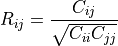
The values of R are between -1 and 1, inclusive.

xarray_like: A 1-D or 2-D array containing multiple variables and observations. Each row of x represents a variable, and each column a single observation of all those variables. Also see rowvar below.
yarray_like, optional: An additional set of variables and observations. y has the same shape as x.
rowvarbool, optional: If rowvar is True (default), then each row represents a variable, with observations in the columns. Otherwise, the relationship is transposed: each column represents a variable, while the rows contain observations.
dtypedata-type, optional: Data-type of the result. By default, the return data-type will have at least numpy.float64 precision.

Added in version 1.20.

Rndarray: The correlation coefficient matrix of the variables.

cov : Covariance matrix

Due to floating point rounding the resulting array may not be Hermitian, the diagonal elements may not be 1, and the elements may not satisfy the inequality abs(a) <= 1. The real and imaginary parts are clipped to the interval [-1, 1] in an attempt to improve on that situation but is not much help in the complex case.

>>> import numpy as np

In this example we generate two random arrays, xarr and yarr, and compute the row-wise and column-wise Pearson correlation coefficients, R. Since rowvar is true by default, we first find the row-wise Pearson correlation coefficients between the variables of xarr.

>>> import numpy as np
>>> rng = np.random.default_rng(seed=42)
>>> xarr = rng.random((3, 3))
>>> xarr
array([[0.77395605, 0.43887844, 0.85859792],
       [0.69736803, 0.09417735, 0.97562235],
       [0.7611397 , 0.78606431, 0.12811363]])
>>> R1 = np.corrcoef(xarr)
>>> R1
array([[ 1.        ,  0.99256089, -0.68080986],
       [ 0.99256089,  1.        , -0.76492172],
       [-0.68080986, -0.76492172,  1.        ]])

If we add another set of variables and observations yarr, we can compute the row-wise Pearson correlation coefficients between the variables in xarr and yarr.

>>> yarr = rng.random((3, 3))
>>> yarr
array([[0.45038594, 0.37079802, 0.92676499],
       [0.64386512, 0.82276161, 0.4434142 ],
       [0.22723872, 0.55458479, 0.06381726]])
>>> R2 = np.corrcoef(xarr, yarr)
>>> R2
array([[ 1.        ,  0.99256089, -0.68080986,  0.75008178, -0.934284  ,
        -0.99004057],
       [ 0.99256089,  1.        , -0.76492172,  0.82502011, -0.97074098,
        -0.99981569],
       [-0.68080986, -0.76492172,  1.        , -0.99507202,  0.89721355,
         0.77714685],
       [ 0.75008178,  0.82502011, -0.99507202,  1.        , -0.93657855,
        -0.83571711],
       [-0.934284  , -0.97074098,  0.89721355, -0.93657855,  1.        ,
         0.97517215],
       [-0.99004057, -0.99981569,  0.77714685, -0.83571711,  0.97517215,
         1.        ]])

Finally if we use the option rowvar=False, the columns are now being treated as the variables and we will find the column-wise Pearson correlation coefficients between variables in xarr and yarr.

>>> R3 = np.corrcoef(xarr, yarr, rowvar=False)
>>> R3
array([[ 1.        ,  0.77598074, -0.47458546, -0.75078643, -0.9665554 ,
         0.22423734],
       [ 0.77598074,  1.        , -0.92346708, -0.99923895, -0.58826587,
        -0.44069024],
       [-0.47458546, -0.92346708,  1.        ,  0.93773029,  0.23297648,
         0.75137473],
       [-0.75078643, -0.99923895,  0.93773029,  1.        ,  0.55627469,
         0.47536961],
       [-0.9665554 , -0.58826587,  0.23297648,  0.55627469,  1.        ,
        -0.46666491],
       [ 0.22423734, -0.44069024,  0.75137473,  0.47536961, -0.46666491,
         1.        ]])